stawave1_fn(beam = 20, wave_height = 1, length =5)25162.65This section provides the functions necessary to calculate the resistance caused by waves
STAWAVE-1 s a simplficied method for ship experiencing limited heave and pitch it was developed by Boom, 2013, and is a practical solution due to its low calculation complexity and relatively small number of variables.
STAWAVE-1 has been validated and can be applied when following conditions are met
ITTC equations: G-1
 stawave1_fn (beam:float, wave_height:float, length:float,
              water_density:float=1026, gravity:float=9.81)
STAWAVE-1 finds the resistance caused by bow waves for ships experiencing low heave and pitch
| Type | Default | Details | |
|---|---|---|---|
| beam | float | the beam of the ship [m] | |
| wave_height | float | Significant wave height of wind waves [m] | |
| length | float | The length of the bow on the water line [m]. See documentation for more details | |
| water_density | float | 1026 | this should be for the current temperature and salinity [kg/m^3] |
| gravity | float | 9.81 | |
| Returns | float | Wave resistance [kg*m/s^2] |
stawave1_fn(beam = 20, wave_height = 1, length =5)25162.65In order to calcualte the force exerted on the vessel by the waves, the wave spectra must be calculate. For this the modified Pierson-Moskowitz spectrum [XXXcitationxxx] algorithm is typically used.
\[S_\eta(\omega) =\frac{A_{fw}}{\omega^5} \textrm{exp}(-\frac{B_{fw}}{\omega^4})\]
\[A_{fw} = 173\frac{H_{W1/3}^2}{T_{01}^4}\]
\[B_{fw} = \frac{691}{T_{01}^4}\]
Where
ITTC equations: 10
modified_pierson_moskowitz_spectrum (omega:float, H_W1_3:float)
| Type | Details | |
|---|---|---|
| omega | float | The circular frequency [rads/s] |
| H_W1_3 | float | Significant wave height of Wind and Swell waves [m] |
| Returns | float | The energy density spectrum at the point omega [s] |
As an example of the modified pierson moskowitz spectrum consider the case below
omega = 1
H_W1_3 = 2.0
T_01 = 5.0

S_eta = modified_pierson_moskowitz_spectrum(omega, H_W1_3)
print(S_eta)0.28499477886766The resistance experienced by the ship from waves is calulated using the below process
Wave transfer function is given by \[R_{wave} = R_{AWRL} + R_{AWML}\]
Where
\[ R_{AWML} = \frac{4 \rho_s g \zeta_A^2B^2}{ L_{pp} }\bar{r}_{aw}(\omega) \]
with
\[\bar{r}_{aw}(\omega) = \bar{\omega}^{b_1} \textrm{exp}\left\{ \frac{b_1}{d_1}(1 - \omega^{-d_1}) \right\} a_1 \textrm{Fr}^{1.5} \textrm{exp}(3.50 \textrm{Fr})\]
\[\bar{\omega} = \frac{\sqrt{\frac{L_{pp}}{g}}\sqrt[3]{k_{yy}}}{1.17 \textrm{Fr}^{-0.143}}\omega\]
\[a_1 = 60.3 C_B^{1.34} \]
\[b_1 = \begin{cases} 11.0 & \bar{\omega}<1 \\ -8.5 & \bar{\omega}\geq1 \end{cases}\]
\[d_1 = \begin{cases} 14.0 & \bar{\omega}<1 \\ -566(\frac{L_{pp}}{B})^{-2.66} & \bar{\omega}\geq1 \end{cases}\]
\[ R_{AWRL} = \frac{1}{2} \rho_s g \zeta_A^2B \alpha_1(\omega) \]
\[ \alpha_1(\omega) = \frac{\pi^2 I_1^2 ( 1.5 k T_M ) }{ \pi^2 I_1^2 ( 1.5 k T_M ) + K_1^2 ( 1.5 k T_M ) }f_1 \]
\[ f_1 = 0.692 \left( \frac{V_S}{\sqrt{T_M g}} \right)^{0.769} + 1.81 C_B^{6.95} \]
once R_{AWRL}$, and \(R_{AWML}\)$ are obtained then the added resistance to the ship can be found by integrating the below equation. \[R_{AWL} = 2\int_{0}^{\infty} \frac{R_{wave}}{\zeta_A^2}S_{\eta}(\omega)d\omega\]
Where the variables of the above equations are
ITTC equations: G-12
 R_AWL (zeta_A:float, B:float, L_pp:float, V_s:float, T_M:float,
        C_B:float, k_yy:float, Fr:float, k:float, rho_s:float=1025,
        g:float=9.81, S_eta:object=None, **kwargs)
| Type | Default | Details | |
|---|---|---|---|
| zeta_A | float | wave amplitude [m] | |
| B | float | ship breadth [m] | |
| L_pp | float | Length between perpendiculars [m] | |
| V_s | float | speed through water [m/s] | |
| T_M | float | draught at midship [m] | |
| C_B | float | block coefficient [dimensionless] | |
| k_yy | float | radius of gyration in the lateral direction [dimensionless] | |
| Fr | float | Froude number [dimensionless] | |
| k | float | circular wave number [rads/m] | |
| rho_s | float | 1025 | water density [kg/m^3] |
| g | float | 9.81 | accerleation due to gravity [m/s^2] |
| S_eta | object | None | A function calculating the wave spectrum |
| kwargs | |||
| Returns | tuple | The added wave resistance, the wave resistance from reflection, the wave resistsance from pitching |
 calculate_R_wave (omega:float, C_B:float, L_pp:float, k_yy:float,
                   Fr:float, zeta_A:float, B:float, k:float, T_M:float,
                   V_s:float, rho_s:float=1025, g:float=9.81)
| Type | Default | Details | |
|---|---|---|---|
| omega | float | circular wave frequency [rads/s] | |
| C_B | float | block coefficient [dimensionless] | |
| L_pp | float | Length between perpendiculars [m] | |
| k_yy | float | radius of gyration in the lateral direction [dimensionless] | |
| Fr | float | Froude number [dimensionless] | |
| zeta_A | float | wave amplitude [m] | |
| B | float | ship breadth [m] | |
| k | float | circular wave number [rads/m] | |
| T_M | float | draught at midship [m] | |
| V_s | float | speed through water [m/s] | |
| rho_s | float | 1025 | water density [kg/m^3] |
| g | float | 9.81 | acceleration due to gravity [m/s^2] |
| Returns | tuple | Function outputs the wave transfer function as well as the component parts R_AWRL and R_AWML |
# Ship parameters
L_pp = 250  # meters
V_s = 10  # meters per second
beaufort_scale = 5
Fr = 0.3

# Example values for other parameters (adjust based on the specific ship)
omega = 0.3 # circular wave frequency [rads/s]
g = 9.81  # m/s^2, force of gravity
k = omega * g # circular wave number [rads/m]
rho_s = 1025  # kg/m^3, water density
zeta_A = 1  # meters, significant wave height
B = 32  # meters, beam of the ship
C_B = 0.7  # block coefficient
T_M = 12  # meters, draught at midship
k_yy = 0.25  # non-dimensional radius of gyration in the lateral direction
I_1 = iv(1, 1.5 * k * T_M)
K_1 = kn(1,  1.5 * k * T_M)


# Calculate R_wave
R_wave = calculate_R_wave(omega, C_B, L_pp, k_yy, Fr, zeta_A, B, k, T_M, V_s, rho_s, g)

R_wave
(229776.13823059603, 128975.85056996053, 100800.2876606355)R_AWL(zeta_A, B, L_pp, V_s, T_M, C_B, k_yy, Fr, k, rho_s, g, S_eta = modified_pierson_moskowitz_spectrum, H_W1_3 = zeta_A)(14670.472278183037, 8072.656348988186, 6597.815929194849)import matplotlib.pyplot as plttransfer_function = lambda omega: (calculate_R_wave(omega = omega, C_B = C_B, L_pp = L_pp, k_yy = k_yy,
Fr = Fr , zeta_A = zeta_A, B = B, k = k, T_M = T_M, V_s = V_s, rho_s = rho_s, g = g))
multipliers = [3, 2, 1, 1/2, 1/4, 1/8]
pierson2 = lambda omega: modified_pierson_moskowitz_spectrum(omega, H_W1_3)
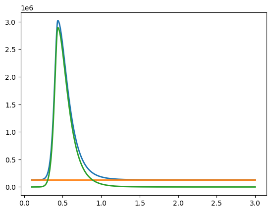
x = np.linspace(0.1, 3, 1000)
y = (np.array([transfer_function(z) for z in x]))
y2 = (np.array([pierson2(z) for z in x]))
fig, ax = plt.subplots()
ax.plot(x, y, linewidth=2.0)
plt.show()