Wind resistance coefficients (wind_res)

datasets of wind coefficients for a range of generic ship types

In order to caluclate the wind resistance experienced by the ship, the wind resistance loading coefficients need to be known. The wind resistance loading coefficients are dependent on the direction the wind is blowing relative to the ship. These coefficients can be found using the following three methods

The first two and fourth approaches are used to create the coefficients specific for the ship. The third option is used when no such simulations have been performed and are based on a set of generic ship designs.

0.1 Load wind resistance coefficients

When there has been no wind tunnel test or CDF analysis the wind resistance coefficients must be found using datasets of look up tables representing generic ship designs for a variety of classes. pyseatrials contains the wind loading factor datasets from ITTC. These data sets have been included as 9 dataframes depending on ship type. To load the data frame enter the name of the ship type to load. The available ship types are

  • GENERAL_CARGO
  • LNG_CARRIER_INT
  • CRUISE_FERRY
  • 280_KDWT_TANKER
  • LNG_CARRIER
  • HANDY_SIZE_BULK_CARRIER
  • 6800_TEU_CONTAINERSHIP
  • MULTI_PURPOSE_CARRIER

source

0.1.1 load_wind_coefficients

 load_wind_coefficients (vessel_type:str)

Load a wind coefficient table for a generic ship class. Datasets from ITTC

Type Details
vessel_type str The name of the vessel type. Must be one of 9 options

Loading a wind resistance dataset for a specific ship type is straight forward if no other dataset is available.

All datasets contain angle of attack in both radians and degrees, the subsequent columns refer to the ship state

general_cargo = load_wind_coefficients("GENERAL_CARGO")

general_cargo
angle_of_attack angle_of_attack_degs average
0 0.000000 0 -0.60
1 0.174533 10 -0.87
2 0.349066 20 -1.00
3 0.523599 30 -1.00
4 0.698132 40 -0.88
5 0.872665 50 -0.85
6 1.047198 60 -0.65
7 1.221730 70 -0.42
8 1.396263 80 -0.27
9 1.570796 90 -0.09
10 1.745329 100 0.09
11 1.919862 110 0.49
12 2.094395 120 0.84
13 2.443461 140 1.39
14 2.617994 150 1.47
15 2.792527 160 1.34
16 2.967060 170 0.92
17 3.141593 180 0.82

0.2 Interpolate the wind loading coefficients

The dataset loaded previously only contains the load coefficients at specific angles. Interpolation is needed to match these coefficients to the wind acting on the ship.There are many ways to interpolate these values, pyseatrials uses simple linear interpolation. Linear interpolation has been chosen over other approaches as it can be vectorised and reduces package dependencies. In addition the ultimate difference, between e.g. linear vs spline interpolation, in resistive force will be small compared to the magnitude of forces acting on the ship.


source

0.2.1 interpolate_cx

 interpolate_cx (df, relative_wind_direction:float, ship_state:str)

Find a linearly interpolated value for wind resistance coefficient

Type Details
df dataframe of the wind resistance dataset
relative_wind_direction float The angle of the wind relative to the ship [rads]
ship_state str The state of the ship the resistance should be evaluated in. Chosen from the columns of the wind resistance datasets
Returns float The dimensionless wind resistance coefficient

Using the example of the general cargo ship using four different wind direction scenarios (0, 55, 180, 280 degrees) we get the interpolated loading coefficients. Some ships have data for different states such as ‘laden’ and ‘ballast’ the General Cargo dataset only has a single state ‘average’.

degs = [0, 55, 120, 180 ]
rads = np.deg2rad(degs) #convert the degrees to radians
cx_vals = interpolate_cx(general_cargo, rads, 'average')
print(cx_vals)
[-0.6  -0.75  0.84  0.82]
import pandas as pd

The wind resistance coefficients can then be used to find the actual wind resistance experienced by the ship

from pyseatrials.general import *
wind_resistance_linear = wind_resistance(air_density = 1.2,
                   wind_resistance_coef_rel = cx_vals,
                   wind_resistance_coef_zero = cx_vals[0],
                   area = 500,
                   relative_wind_speed = 20,
                   sog = 10)

#convert to kN
resistance_linear_kN = np.round(wind_resistance_linear/1000)
print(resistance_linear_kN )
[-54. -72. 119. 116.]

Other interpolations methods can be used such as spline interpolation from the scipy library.

from scipy.interpolate import make_interp_spline
cx_spline = make_interp_spline(general_cargo['angle_of_attack'], general_cargo['average'] )

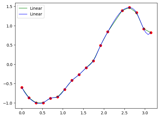
The difference between the load coefficients produced by the two models can be shown in the plot below. Across the full range there is almost no difference.

import matplotlib.pyplot as plt
xs = np.linspace(-3, 3, 100)
xvals = np.linspace(0, np.pi, 50)
yinterp_lin = np.interp(xvals, general_cargo['angle_of_attack'], general_cargo['average'])
yinterp_spline = cx_spline(xvals)
plt.plot(general_cargo['angle_of_attack'], general_cargo['average'], 'ro')
plt.plot(xvals, yinterp_lin,'g-', lw=1, label='Linear')
plt.plot(xvals, yinterp_spline,'b-', lw=1, label='Linear')
plt.legend(loc='best')
plt.show()

The difference in terms of actual resistive force between linear and spline interpolation is also very small.

wind_resistiance_spline = wind_resistance(air_density = 1.2,
                   wind_resistance_coef_rel = cx_spline(rads),
                   wind_resistance_coef_zero = cx_spline(rads)[0],
                   area = 500,
                   relative_wind_speed = 20,
                   sog = 10)
#convert to kN
resitance_spline_kN = np.round(wind_resistiance_spline/1000)

#difference in wind resistance between the two models in kN
print('difference in kN between the two interpolation methods for all 4 angles of attack '+str(resistance_linear_kN - resitance_spline_kN))
difference in kN between the two interpolation methods for all 4 angles of attack [0. 2. 0. 0.]

1 Fujiwara regression formula

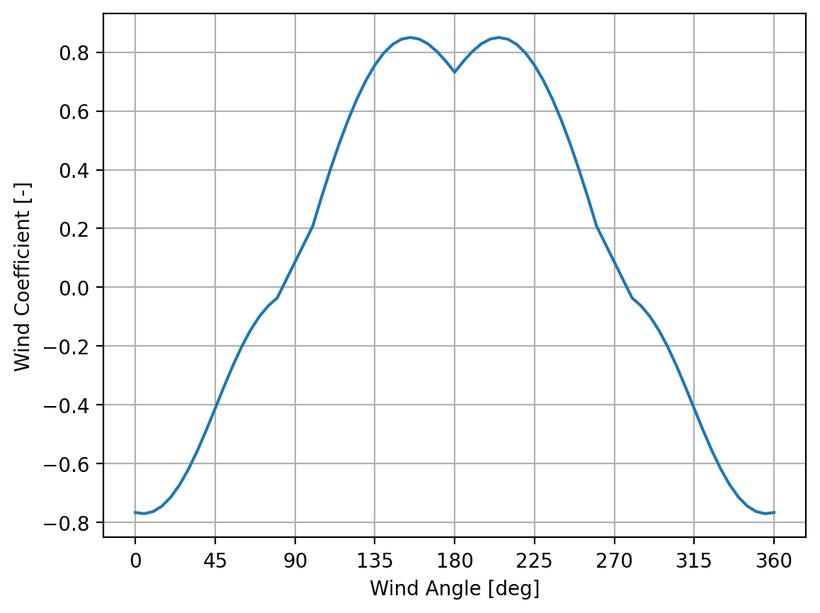
The Fujiwara regression formula (Fujiwara 2006) calcualtes the wind resistance coeficient of a vessel using the ships geometry. It is often considered the default method, due to it’s adaptability to specific ships and the accessability of the input parameters. However, it’s input calculation is somewhat involved, we reccomend reading either the ITTC or ISO15016 Standards for detailed description of its application.

\[C_{DA} = C_{LF}cos \psi_{WR} + C_{XLI}\left(sin \psi_{WR} - \frac{1}{2}sin \psi_{WR}cos^2 \psi_{WR} \right) sin \psi_{WR}cos \psi_{WR} +C_{ALF}sin \psi_{WR}cos^3 \psi_{WR}\]

with

for \[0 \leq \psi_{WR} < 90 [deg]\]

\[ C_{LF} = \beta_{10} + \beta_{11} \frac{A_{LV}}{L_{OA}B} + \beta_{12} \frac{C_{MC}}{L_{OA}} \]

\[ C_{XLI} = \delta_{10} + \delta_{11} \frac{A_{LV}}{L_{OA}h_{BR}} + \delta_{12} \frac{A_{XV}}{Bh_{BR}} \]

\[ C_{ALF} = \epsilon_{10} + \epsilon_{11} \frac{A_{OD}}{A_{LV}} + \epsilon_{12} \frac{B}{L_{OA}} \]

for \[90 < \psi_{WR} \leq 180 [deg]\]

\[ C_{LF} = \beta_{20} + \beta_{21} \frac{B}{L_{OA}} + \beta_{22} \frac{h_C}{L_{OA}} + \beta_{23} \frac{A_{OD}}{{L_{OA}}^2} + \beta_{24} \frac{A_{XV}}{B^2} \]

\[ C_{XLI} = \delta_{20} + \delta_{21} \frac{A_{LV}}{L_{OA}h_{BR}} + \delta_{22} \frac{A_{XV}}{A_{LV}} + \delta_{23} \frac{B}{L_{OA}} + \delta_{24} \frac{A_{XV}}{Bh_{BR}} \]

\[ C_{ALF} = \epsilon_{20} + \epsilon_{21} \frac{A_{OD}}{A_{LV}} \]

for \[ \psi_{WR} = 90 [deg]\]

\[ C_{DA| \psi_{WR}=90[deg]} = \frac{1}{2} \left(C_{DA| \psi_{WR}=90[deg] - \mu} + C_{DA| \psi_{WR}=90[deg] + \mu} \right) \]

Where

\(A_{OD}\) is the lateral projected area of superstructures on deck \([m^2]\),

$ A_{XV} $ is the area of maximum transverse section exposed to the winds $ [m^2] $,

\(A_{LV}\) is the projected lateral area above the waterline \([m^2]\),

$ B $ is the ship breadth $ [m] $,

$ C_{DA} $ is the wind resistance coefficient [-]

$ C_{MC} $ is the horizontal distance from midship section to centre of lateral projected area $ A_{LV} $, $ [m^2] $. This is often negative,

$ h_{BR} $ is the height of top of superstructure (bridge etc) $ [m] $,

$ h_c $ is the height from the waterline to the centre of lateral projected area $ A_{LV} $, $ [m] $,

$ L_{OA} $ is the length overall $ [m] $,

$ $ is the smoothing range, normally 10 $ [deg] $,

$ _{WR} $ is the relative wind direction $ [deg] $. 0 means head winds

The non-dimensional parameters $ {ij}, {ij}  and  _{ij} $ used are shown in the table below

i j
0 1 2 3 4
$ _{ij} $ 1 0.922 -0.507 -1.162 - -
2 -0.018 5.091 -10.367 3.011 0.341
$ _{ij} $ 1 -0.458 -3.245 2.313 - -
2 1.901 -12.727 -24.407 40.310 5.481
$ _{ij} $ 1 0.585 0.906 -3.239 - -
2 0.314 1.117 0 0 0

ITTC equations: F-1 to F-7

\(A_{LV}\) is the projected lateral area above the waterline \(\[m^2\]\),

$ B $ is the ship breadth $ [m] $,

$ C_{DA} $ is the wind resistance coefficient [-]

$ C_{MC} $ is the horizontal distance from midship section to centre of lateral projected area $ A_{LV} $, $ [m^2] $. This is often negative,

$ h_{BR} $ is the height of top of superstructure (bridge etc) $ [m] $,

$ h_c $ is the height from the waterline to the centre of lateral projected area $ A_{LV} $, $ [m] $,

$ L_{OA} $ is the length overall $ [m] $,

$ $ is the smoothing range, normally 10 $ [deg] $,

$ _{WR} $ is the relative wind direction $ [deg] $. 0 means head winds

The non-dimensional parameters $ {ij}, {ij}  and  _{ij} $ used are shown in the table below

i j
0 1 2 3 4
$ _{ij} $ 1 0.922 -0.507 -1.162 - -
2 -0.018 5.091 -10.367 3.011 0.341
$ _{ij} $ 1 -0.458 -3.245 2.313 - -
2 1.901 -12.727 -24.407 40.310 5.481
$ _{ij} $ 1 0.585 0.906 -3.239 - -
2 0.314 1.117 0 0 0

ITTC equations: F-1 to F-7


source

1.0.1 fujiwara

 fujiwara (aod:float, axv:float, alv:float, cmc:float, hc:float,
           hbr:float, loa:float, b:float, wind_dir:float,
           smoothing:float=10)
Type Default Details
aod float is the lateral projected area of superstructures on deck [m2]
axv float is the area of maximum transverse section exposed to the winds [m2]
alv float is the projected lateral area above the waterline [m2]
cmc float is the horizontal distance from midship section to centre of lateral projected area ALV, this is often negative. [m2]
hc float is the height from the waterline to the centre of lateral projected area ALV [m]
hbr float is the height of top of superstructure (bridge etc) [m]
loa float is the length overall [m]
b float is the ship breadth [m]
wind_dir float is the relative wind direction, 0 means head winds. [deg]
smoothing float 10 is the smoothing range, normally 10 degrees. [deg]
Returns float returns the wind coefficient in the longitudinal direction [-]
import matplotlib.pyplot as plt
wind_dir = np.arange(0, 361, 5)

cx = [fujiwara(aod = 905, axv = 1750, alv = 7400, cmc = -6.6, hc = 11.72, hbr = 40.7, loa = 340, b = 62, wind_dir = i, smoothing = 10) for i in wind_dir]
plt.plot(wind_dir, cx)
plt.xlabel('Wind Angle [deg]')
plt.ylabel('Wind Coefficient [-]')
plt.xticks(np.arange(0,361,45))
plt.grid()